Examples
otargen.Rmd1. Retrieve colocalisation data for one or more
genes:
In this example, we retrieve colocalization data for one or more genes of interest. The data provides evidence that if genetic variants which are linked to both molecular traits and traits within shared genomic regions are identical. By utilizing the otargen , we can investigate these colocalization patterns and gain valuable insights for further analysis and interpretation.
library(otargen)


# Specify the genes of interest
genes_of_interest <- c("ENSG00000163946", "ENSG00000169174", "ENSG00000143001")

# Retrieve colocalization data
coloc_data <- colocalisationsForGene(genes = genes_of_interest)

head(coloc_data)

# A tibble: 668 × 20
   Study    Trait_reported Lead_variant Molecular_trait Gene_symbol Tissue Source    H3    H4   `log2(H4/H3)`
   <chr>    <chr>          <chr>        <chr>           <chr>       <chr>  <chr>  <dbl> <dbl>         <dbl>
 1 GCST900… Mean platelet… 3_56619974_… TASOR           ENSG000001… blood  Lepik…     0     1         17.3
 2 GCST900… Direct low de… 1_55029009_… PCSK9           ENSG000001… iPSC   PhLiPS     0     1         11.4
 3 GCST900… Direct low de… 1_55029009_… PCSK9           ENSG000001… iPSC   iPSCO…     0     1         11.3
 4 GCST900… Direct low de… 1_55029009_… PCSK9           ENSG000001… iPSC   HipSci     0     1         11.3
 5 GCST900… High choleste… 1_55025188_… PCSK9           ENSG000001… tibia… GTEx-…     0     1         10.7
 6 NEALE2_… Yes, because … 1_55026242_… PCSK9           ENSG000001… tibia… GTEx-…     0     1         10.4
 7 SAIGE_2… Hyperlipidemia 1_55023869_… PCSK9           ENSG000001… lung   GTEx-…     0     1          9.82
 8 SAIGE_2… Hypercholeste… 1_55023869_… PCSK9           ENSG000001… lung   GTEx-…     0     1          9.79
 9 SAIGE_2… Disorders of … 1_55023869_… PCSK9           ENSG000001… lung   GTEx-…     0     1          9.77
10 SAIGE_2… Hyperlipidemia 1_55023869_… PCSK9           ENSG000001… tibia… GTEx-…     0     1          9.77
# ℹ 658 more rows
# ℹ 10 more variables: Title <chr>, Author <chr>, Has_sumstats <lgl>, numAssocLoci <dbl>,
#   `nInitial cohort` <dbl>, study_nReplication <dbl>, study_nCases <dbl>, Publication_date <chr>,
#   Journal <chr>, Pubmed_id <chr>
2. Retrieve QTL credible set data
In this example, we utilize the qtlCredibleSet()
function to fetch the credible set of tag variants. By specifying the
study ID, variant ID, gene, and
biofeature, we extract valuable information about the tag
variants with a high probability of being associated with the trait of
interest.
# Retrieve QTL credible set data
qtl_cred_set <- qtlCredibleSet(studyid = "Braineac2", variantid = "rs7552841",
                              gene = "PCSK9", biofeature = "SUBSTANTIA_NIGRA")

# Display the first few rows of the QTL credible set data
head(qtl_cred_set)


   tagVariant.id tagVariant.rsId        pval       se      beta    postProb MultisignalMethod   logABF is95 is99
1 1_55052794_A_G              NA 0.000151568 0.166373 -0.681090 0.002299181       conditional 2.726953 TRUE TRUE
2 1_55054539_G_A              NA 0.000482125 0.193346  0.721143 0.001422319       conditional 2.246689 TRUE TRUE
3 1_55241800_A_G              NA 0.000634235 0.181505  0.660898 0.001326061       conditional 2.176614 TRUE TRUE
4 1_55246294_A_G              NA 0.000527554 0.181065  0.670092 0.001424974       conditional 2.248554 TRUE TRUE
5 1_55248288_C_T              NA 0.000650165 0.182720  0.663849 0.001293980       conditional 2.152124 TRUE TRUE
6 1_55248542_G_A              NA 0.000650880 0.182789  0.664035 0.001293430       conditional 2.151698 TRUE TRUE
3. Retrieves L2G model summary data for
gene(s).
In this exemplary usage, we demonstrate the application of the
studiesAndLeadVariantsForGeneByL2G() function to obtain one
of the core data tables provided by Open Target Genetics. The function
utilizes the powerful “locus-to-gene” (L2G) model, which leverages
genetic and functional genomics features to prioritize likely causal
genes at each GWAS locus. By specifying the gene of interest and
applying customized filters, we retrieve prioritization scores for the
lead variants associated with our specified genes, as well as other
genes sharing the same loci. The resulting data table is presented in
the tidy and comprehensive tibble format, encompassing a wealth of
scores and information pertaining to the L2G model, genetic variants,
associated studies, and more. By conducting further analysis on these
results, we can delve deeper into the intricate relationships between
genes and traits, leading to groundbreaking insights and
discoveries.
# Retrieve L2G results for the gene PCSK9 with specified filters
l2g_results <- studiesAndLeadVariantsForGeneByL2G(
  genes = "PCSK9",
  l2g = 0.6,
  pvalue = 1e-8,
  vtype = c("intergenic_variant", "intron_variant")
)

# Display the results as a tibble for easier analysis
l2g_results %>% as_tibble()

# A tibble: 40 × 39
   yProbaModel yProbaDistance yProbaInteraction yProbaMolecularQTL yProbaPathogenicity     pval beta.direction beta.betaCI
         <dbl>          <dbl>             <dbl>              <dbl>               <dbl>    <dbl> <chr>                <dbl>
 1       0.618          0.544             0.056              0.221               0.615 4.79e-12 +                   0.394
 2       0.631          0.761             0.284              0.155               0.058 5.23e-20 -                  -0.0687
 3       0.631          0.757             0.284              0.155               0.058 3.54e-20 -                  -0.0668
 4       0.647          0.739             0.25               0.138               0.182 3   e-47 -                  -0.0544
 5       0.652          0.614             0.171              0.637               0.344 3.60e-14 +                   0.0156
 6       0.656          0.765             0.284              0.279               0.058 1.13e-41 -                  -0.069
 7       0.656          0.765             0.284              0.279               0.058 2.38e-53 -                  -0.0831
 8       0.66           0.69              0.171              0.487               0.047 1   e- 8 -                  NA
 9       0.663          0.756             0.206              0.33                0.056 1   e-10 -                  -0.03
10       0.664          0.767             0.206              0.614               0.057 1.90e-88 -                  -0.0487
# ℹ 30 more rows
# ℹ 31 more variables: beta.betaCILower <dbl>, beta.betaCIUpper <dbl>, odds.oddsCI <dbl>, odds.oddsCILower <dbl>,
#   odds.oddsCIUpper <dbl>, study.studyId <chr>, study.traitReported <chr>, study.traitCategory <chr>, study.pubDate <chr>,
#   study.pubTitle <chr>, study.pubAuthor <chr>, study.pubJournal <chr>, study.pmid <chr>, study.hasSumstats <lgl>,
#   study.nCases <int>, study.numAssocLoci <int>, study.nTotal <int>, study.traitEfos <chr>, variant.id <chr>, variant.rsId <chr>,
#   variant.chromosome <chr>, variant.position <int>, variant.refAllele <chr>, variant.altAllele <chr>,
#   variant.nearestCodingGeneDistance <int>, variant.nearestGeneDistance <int>, variant.mostSevereConsequence <chr>, …
from Open Target Genetics portal
Interpreting the L2G score The L2G model produces a score, ranging from 0 to 1, which reflects the approximate fraction of GSP genes among all genes near a given threshold. This can be interpreted to say that genes with an L2G score of 0.5 have a 50% chance of being the causal gene at the locus, under the assumption that the model is correct and the locus itself is similar to those in our gold-standard training data. Note: Because models don’t generalize perfectly, the true fraction of causal genes at an L2G score of 0.5 is likely to be less than 50%. A key strength of the L2G score is that it aggregates information over all credible set variants, rather than looking only at the distance from the lead GWAS variant to genes.
4. Obtain detailed information about all the genes present in
a given region of a specified chromosome.
The genes query type in the Open Target Genetics
GraphQL schema provides a convenient way to retrieve all
the genes within a specific genomic region by supplying positional
information. The wrapper function getLociGenes() in the
otargen package allows you to execute this query and obtain
a tidy table to gain insights into the genes located within the
specified genomic region.
# Retrieve genes within a genomic region on chromosome 2
genes_table <- getLociGenes(chromosome = "2", start = 239634984, end = 241634984)

# Display the resulting table
genes_table


# A tibble: 27 × 10
   id              symbol  bioType        description                                   chromosome    tss  start    end fwdStrand exons
   <chr>           <chr>   <chr>          <chr>                                         <chr>       <int>  <int>  <int> <lgl>     <lis>
 1 ENSG00000006607 FARP2   protein_coding FERM, ARH/RhoGEF and pleckstrin domain prote… 2          2.41e8 2.41e8 2.41e8 TRUE      <int>
 2 ENSG00000063660 GPC1    protein_coding glypican 1 [Source:HGNC Symbol;Acc:HGNC:4449] 2          2.40e8 2.40e8 2.40e8 TRUE      <int>
 3 ENSG00000115677 HDLBP   protein_coding high density lipoprotein binding protein [So… 2          2.41e8 2.41e8 2.41e8 FALSE     <int>
 4 ENSG00000115685 PPP1R7  protein_coding protein phosphatase 1 regulatory subunit 7 [… 2          2.41e8 2.41e8 2.41e8 TRUE      <int>
 5 ENSG00000115687 PASK    protein_coding PAS domain containing serine/threonine kinas… 2          2.41e8 2.41e8 2.41e8 FALSE     <int>
 6 ENSG00000115694 STK25   protein_coding serine/threonine kinase 25 [Source:HGNC Symb… 2          2.42e8 2.41e8 2.42e8 FALSE     <int>
 7 ENSG00000122085 MTERF4  protein_coding mitochondrial transcription termination fact… 2          2.41e8 2.41e8 2.41e8 FALSE     <int>
 8 ENSG00000130294 KIF1A   protein_coding kinesin family member 1A [Source:HGNC Symbol… 2          2.41e8 2.41e8 2.41e8 FALSE     <int>
 9 ENSG00000130414 NDUFA10 protein_coding NADH:ubiquinone oxidoreductase subunit A10 [… 2          2.40e8 2.40e8 2.40e8 FALSE     <int>
10 ENSG00000142327 RNPEPL1 protein_coding arginyl aminopeptidase like 1 [Source:HGNC S… 2          2.41e8 2.41e8 2.41e8 TRUE      <int>
# ℹ 17 more rows
# ℹ Use `print(n = ...)` to see more rows
5. Plot data obtained from the manhattan() function.
A Manhattan plot is commonly used to visualize GWAS summary data. It
displays the p-values (-log10(P)) of genetic variants across the genome,
typically plotted against their respective chromosomal positions.
manhattan() is the wrapper function in otargen
to retrieve variants summary statistics for a GWAS study. Now, it is not
easy to go through the large table of variants and see which variants
has the most significant association, on the other hand, writing a nice
looking code to render a Manhatan plot can be time consuming.
plot_manhatan() in otargen dose the job and
all you need is to pipe the manhatan() output to it.
Here’s an example code snippet:
manhattan(studyid = "GCST003044") %>% plot_manhattan()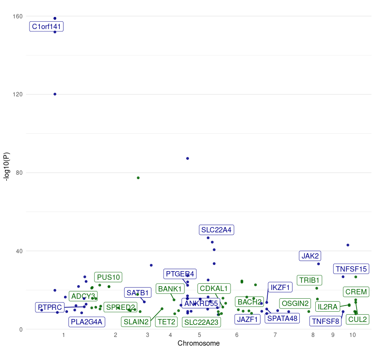
6. Plot data obtained from the PheWAS() function.
A Phenome-Wide Association Study (PheWAS) analyzes the association
between genetic variants and a wide range of phenotypic traits. To
retrieve PheWAS analysis results for a variant, you can use
pheWAS() function in otargen which returns a
tidy data table of all calculated statistics for association of the
specified variant across many traits in UK Biobank,
FinnGen, ’ and or GWAS Catalog. Now, as shown in below
example snippet piping, output of pheWAS() to
plot_phewas() will return you a nice scatter plot with
useful color codes to interpret those associations! It is even more fun,
that the plot allows to choose if you are only interested to keep
disease associated variants in the plot.
pheWAS(variantid = "14_87978408_G_A") %>% plot_phewas(disease = TRUE)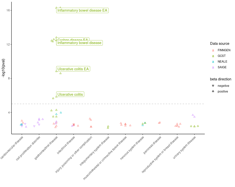
**7. Plot the scores obtained from the *studiesAndLeadVariantsForGeneByL2G()**
In Example 3 we talked about
studiesAndLeadVariantsForGeneByL2G() that returns a
comprehensive data tables of L2G model statistics. Now using
plot_l2g() allows you to generate pretty radar plots to
compare the partial scores from L2G model between the list of genes that
you are interested to priotise using these scores. In addition,
plot_l2g() allows to plot only for specific disease by
specifying a corresponding EFO id for disease
parameter.
``` r # Retrieve L2G model statistics for a list of genes l2g_results <- studiesAndLeadVariantsForGeneByL2G(list(“ENSG00000167207”,“ENSG00000096968”,“ENSG00000138821”, “ENSG00000125255”))
